SEO Analytics for Free – Combining Google Search with the Moz API

I’m a self-funded start-up business owner. As such, I want to get as much as I can for free before convincing our finance director to spend our hard-earned bootstrapping funds. I’m also an analyst with a background in data and computer science, so a bit of a geek by any definition.

What I try to do, with my SEO analyst hat on, is hunt down great sources of free data and wrangle it into something insightful. Why? Because there’s no value in basing client advice on conjecture. It’s far better to combine quality data with good analysis and help our clients better understand what’s important for them to focus on.

In this article, I will tell you how to get started using a few free resources and illustrate how to pull together unique analytics that provide useful insights for your blog articles if you’re a writer, your agency if you’re an SEO, or your website if you’re a client or owner doing SEO yourself.

The scenario I’m going to use is that I want analyze some SEO attributes (e.g. backlinks, Page Authority etc.) and look at their effect on Google ranking. I want to answer questions like “Do backlinks really matter in getting to Page 1 of SERPs?” and “What kind of Page Authority score do I really need to be in the top 10 results?” To do this, I will need to combine data from a number of Google searches with data on each result that has the SEO attributes in that I want to measure.

Let’s get started and work through how to combine the following tasks to achieve this, which can all be setup for free:

• Querying with Google Custom Search Engine
• Using the free Moz API account
• Harvesting data with PHP and MySQL
• Analyzing data with SQL and R

Querying with Google Custom Search Engine

We first need to query Google and get some results stored. To stay on the right side of Google’s terms of service, we’ll not be scraping Google.com directly but will instead use Google’s Custom Search feature. Google’s Custom Search is designed mainly to let website owners provide a Google like search widget on their website. However, there is also a REST based Google Search API that is free and lets you query Google and retrieve results in the popular JSON format. There are quota limits but these can be configured and extended to provide a good sample of data to work with.

When configured correctly to search the entire web, you can send queries to your Custom Search Engine, in our case using PHP, and treat them like Google responses, albeit with some caveats. The main limitations of using a Custom Search Engine are: (i) it doesn’t use some Google Web Search features such as personalized results and; (ii) it may have a subset of results from the Google index if you include more than ten sites.

Notwithstanding these limitations, there are many search options that can be passed to the Custom Search Engine to proxy what you might expect Google.com to return. In our scenario, we passed the following when making a call:

https://www.googleapis.com/customsearch/v1?key=&userIp=
&cx&q=iPhone+X&cr=countryUS&start=
1

Where:

• https://www.googleapis.com/customsearch/v1 – is the URL for the Google Custom Search API
• key= – Your Google Developer API Key
• userIp= – The IP address of the local machine making the call
• cx= – Your Google Custom Search Engine ID
• q=iPhone+X – The Google query string (‘+’ replaces ‘ ‘)
• cr=countryUS – Country restriction (from Goolge’s Country Collection Name list)
• start=1 – The index of the first result to return – e.g. SERP page 1. Successive calls would increment this to get pages 2–5.

Google has said that the Google Custom Search engine differs from Google .com, but in my limited prod testing comparing results between the two, I was encouraged by the similarities and so continued with the analysis. That said, keep in mind that the data and results below come from Google Custom Search (using ‘whole web’ queries), not Google.com.

Using the free Moz API account

Moz provide an Application Programming Interface (API). To use it you will need to register for a Mozscape API key, which is free but limited to 2,500 rows per month and one query every ten seconds. Current paid plans give you increased quotas and start at $250/month. Having a free account and API key, you can then query the Links API and analyze the following metrics:

NOTE: Since this analysis was captured, Moz documented that they have deprecated these fields. However, in testing this (15-06-2019), the fields were still present.

Moz API Codes are added together before calling the Links API with something that looks like the following:

www.apple.com%2F?Cols=103616137253&AccessID=MOZ_ACCESS_ID&
Expires=1560586149&Signature=

Where:

• http://lsapi.seomoz.com/linkscape/url-metrics/” class=”redactor-autoparser-object”>http://lsapi.seomoz.com/linksc… – Is the URL for the Moz API
• http%3A%2F%2Fwww.apple.com%2F – An encoded URL that we want to get data on
• Cols=103616137253 – The sum of the Moz API codes from the table above
• AccessID=MOZ_ACCESS_ID – An encoded version of the Moz Access ID (found in your API account)
• Expires=1560586149 – A timeout for the query – set a few minutes into the future
• Signature= – An encoded version of the Moz Access ID (found in your API account)

Moz will return with something like the following JSON:

Array
(
    [ut] => Apple
    [uu] => www.apple.com/
    [ueid] => 13078035
    [uid] => 14632963
    [uu] => www.apple.com/
    [ueid] => 13078035
    [uid] => 14632963
    [umrp] => 9
    [umrr] => 0.8999999762
    [fmrp] => 2.602215052
    [fmrr] => 0.2602215111
    [us] => 200
    [upa] => 90
    [pda] => 100
)

For a great starting point on querying Moz with PHP, Perl, Python, Ruby and Javascript, see this repository on Github. I chose to use PHP.

Harvesting data with PHP and MySQL

Now we have a Google Custom Search Engine and our Moz API, we’re almost ready to capture data. Google and Moz respond to requests via the JSON format and so can be queried by many popular programming languages. In addition to my chosen language, PHP, I wrote the results of both Google and Moz to a database and chose MySQL Community Edition for this. Other databases could be also used, e.g. Postgres, Oracle, Microsoft SQL Server etc. Doing so enables persistence of the data and ad-hoc analysis using SQL (Structured Query Language) as well as other languages (like R, which I will go over later). After creating database tables to hold the Google search results (with fields for rank, URL etc.) and a table to hold Moz data fields (ueid, upa, uda etc.), we’re ready to design our data harvesting plan.

Google provide a generous quota with the Custom Search Engine (up to 100M queries per day with the same Google developer console key) but the Moz free API is limited to 2,500. Though for Moz, paid for options provide between 120k and 40M rows per month depending on plans and range in cost from $250–$10,000/month. Therefore, as I’m just exploring the free option, I designed my code to harvest 125 Google queries over 2 pages of SERPs (10 results per page) allowing me to stay within the Moz 2,500 row quota. As for which searches to fire at Google, there are numerous resources to use from. I chose to use Mondovo as they provide numerous lists by category and up to 500 words per list which is ample for the experiment.

I also rolled in a few PHP helper classes alongside my own code for database I/O and HTTP.

In summary, the main PHP building blocks and sources used were:

One factor to be aware of is the 10 second interval between Moz API calls. This is to prevent Moz being overloaded by free API users. To handle this in software, I wrote a “query throttler” which blocked access to the Moz API between successive calls within a timeframe. However, whilst working perfectly it meant that calling Moz 2,500 times in succession took just under 7 hours to complete.

Analyzing data with SQL and R

Data harvested. Now the fun begins!

It’s time to have a look at what we’ve got. This is sometimes called data wrangling. I use a free statistical programming language called R along with a development environment (editor) called R Studio. There are other languages such as Stata and more graphical data science tools like Tableau, but these cost and the finance director at Purple Toolz isn’t someone to cross!

I have been using R for a number of years because it’s open source and it has many third-party libraries, making it extremely versatile and appropriate for this kind of work.

Let’s roll up our sleeves.

I now have a couple of database tables with the results of my 125 search term queries across 2 pages of SERPS (i.e. 20 ranked URLs per search term). Two database tables hold the Google results and another table holds the Moz data results. To access these, we’ll need to do a database INNER JOIN which we can easily accomplish by using the RMySQL package with R. This is loaded by typing “install.packages(‘RMySQL’)” into R’s console and including the line “library(RMySQL)” at the top of our R script.

We can then do the following to connect and get the data into an R data frame variable called “theResults.”

library(RMySQL)
# INNER JOIN the two tables
theQuery <- "
    SELECT A.*, B.*, C.*
    FROM
    (
        SELECT 
            cseq_search_id
        FROM cse_query
    ) A -- Custom Search Query
    INNER JOIN
    (
        SELECT 
            cser_cseq_id,
            cser_rank,
            cser_url
        FROM cse_results
    ) B -- Custom Search Results
    ON A.cseq_search_id = B.cser_cseq_id
    INNER JOIN
    (
        SELECT *
        FROM moz
    ) C -- Moz Data Fields
    ON B.cser_url = C.moz_url
    ;
"
# [1] Connect to the database
# Replace USER_NAME with your database username
# Replace PASSWORD with your database password
# Replace MY_DB with your database name
theConn <- dbConnect(dbDriver("MySQL"), user = "USER_NAME", password = "PASSWORD", dbname = "MY_DB")
# [2] Query the database and hold the results
theResults <- dbGetQuery(theConn, theQuery)
# [3] Disconnect from the database
dbDisconnect(theConn)

NOTE: I have two tables to hold the Google Custom Search Engine data. One holds data on the Google query (cse_query) and one holds results (cse_results).

We can now use R’s full range of statistical functions to begin wrangling.

Let’s start with some summaries to get a feel for the data. The process I go through is basically the same for each of the fields, so let’s illustrate and use Moz’s ‘UEID’ field (the number of external equity links to a URL). By typing the following into R I get the this:

> summary(theResults$moz_ueid)
   Min. 1st Qu.  Median    Mean 3rd Qu.    Max. 
      0       1      20   14709     182 2755274 
> quantile(theResults$moz_ueid,  probs = c(1, 5, 10, 25, 50, 75, 80, 90, 95, 99, 100)/100)
       1%        5%       10%       25%       50%       75%       80%       90%       95%       99%      100% 
      0.0       0.0       0.0       1.0      20.0     182.0     337.2    1715.2    7873.4  412283.4 2755274.0 

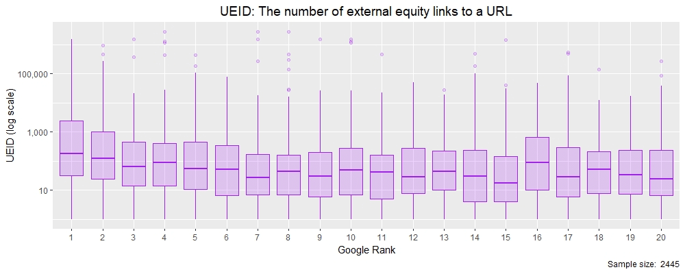
Looking at this, you can see that the data is skewed (a lot) by the relationship of the median to the mean, which is being pulled by values in the upper quartile range (values beyond 75% of the observations). We can however, plot this as a box and whisker plot in R where each X value is the distribution of UEIDs by rank from Google Custom Search position 1-20.

Note we are using a log scale on the y-axis so that we can display the full range of values as they vary a lot!

Box and whisker plots are great as they show a lot of information in them (see the geom_boxplot function in R). The purple boxed area represents the Inter-Quartile Range (IQR) which are the values between 25% and 75% of observations. The horizontal line in each ‘box’ represents the median value (the one in the middle when ordered), whilst the lines extending from the box (called the ‘whiskers’) represent 1.5x IQR. Dots outside the whiskers are called ‘outliers’ and show where the extents of each rank’s set of observations are. Despite the log scale, we can see a noticeable pull-up from rank #10 to rank #1 in median values, indicating that the number of equity links might be a Google ranking factor. Let’s explore this further with density plots.

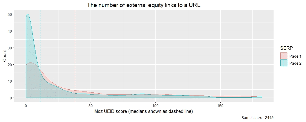
Density plots are a lot like distributions (histograms) but show smooth lines rather than bars for the data. Much like a histogram, a density plot’s peak shows where the data values are concentrated and can help when comparing two distributions. In the density plot below, I have split the data into two categories: (i) results that appeared on Page 1 of SERPs ranked 1-10 are in pink and; (ii) results that appeared on SERP Page 2 are in blue. I have also plotted the medians of both distributions to help illustrate the difference in results between Page 1 and Page 2.

The inference from these two density plots is that Page 1 SERP results had more external equity backlinks (UEIDs) on than Page 2 results. You can also see the median values for these two categories below which clearly shows how the value for Page 1 (38) is far greater than Page 2 (11). So we now have some numbers to base our SEO strategy for backlinks on.

# Create a factor in R according to which SERP page a result (cser_rank) is on
> theResults$rankBin  theResults$rankBin  tapply(theResults$moz_ueid, theResults$rankBin, median) 
Page 1 Page 2 
    38     11 

From this, we can deduce that equity backlinks (UEID) matter and if I were advising a client based on this data, I would say they should be looking to get over 38 equity-based backlinks to help them get to Page 1 of SERPs. Of course, this is a limited sample and more research, a bigger sample and other ranking factors would need to be considered, but you get the idea.

Now let’s investigate another metric that has less of a range on it than UEID and look at Moz’s UPA measure, which is the likelihood that a page will rank well in search engine results.

> summary(theResults$moz_upa)
   Min. 1st Qu.  Median    Mean 3rd Qu.    Max. 
   1.00   33.00   41.00   41.22   50.00   81.00 
> quantile(theResults$moz_upa,  probs = c(1, 5, 10, 25, 50, 75, 80, 90, 95, 99, 100)/100)
  1%   5%  10%  25%  50%  75%  80%  90%  95%  99% 100% 
  12   20   25   33   41   50   53   58   62   75   81 

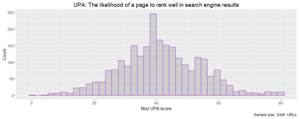
UPA is a number given to a URL and ranges between 0–100. The data is better behaved than the previous UEID unbounded variable having its mean and median close together making for a more ‘normal’ distribution as we can see below by plotting a histogram in R.

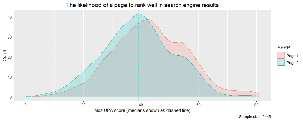
We’ll do the same Page 1 : Page 2 split and density plot that we did before and look at the UPA score distributions when we divide the UPA data into two groups.

# Report the medians by SERP page by calling ‘tapply’
> tapply(theResults$moz_upa, theResults$rankBin, median) 
Page 1 Page 2 
    43     39 

In summary, two very different distributions from two Moz API variables. But both showed differences in their scores between SERP pages and provide you with tangible values (medians) to work with and ultimately advise clients on or apply to your own SEO.

Of course, this is just a small sample and shouldn’t be taken literally. But with free resources from both Google and Moz, you can now see how you can begin to develop analytical capabilities of your own to base your assumptions on rather than accepting the norm. SEO ranking factors change all the time and having your own analytical tools to conduct your own tests and experiments on will help give you credibility and perhaps even a unique insight on something hitherto unknown.

Google provide you with a healthy free quota to obtain search results from. If you need more than the 2,500 rows/month Moz provide for free there are numerous paid-for plans you can purchase. MySQL is a free download and R is also a free package for statistical analysis (and much more).

Go explore!